Power-grid neural solvers are moving beyond one grid, one task.

Power flow, optimal power flow, and state estimation answer different questions. Power flow calculates the electrical state produced by specified injections and controls. Optimal power flow, or OPF, chooses controls such as generator setpoints to minimize an objective while satisfying that electrical state. State estimation reconstructs the state from incomplete and noisy measurements. A model that predicts load or wind may supply an input to those calculations; it is not itself a solver.

The demanding target is alternating-current optimal power flow, or AC-OPF. Its output has to balance active and reactive power at every bus while respecting generator capability, voltage bounds, line thermal limits, transformer settings, and voltage-angle limits. The power-flow equations are nonlinear and the optimization is nonconvex, so a conventional solver can find a strong local solution without proving that no better operating point exists anywhere in the feasible region.

Security-constrained versions repeat that work across equipment failures and other contingencies. Multi-period versions add ramping, storage, and time-coupled decisions. Unit commitment adds discrete start and stop choices. “Grid optimization” therefore names a family of problems, and a neural result on a single steady-state AC-OPF benchmark does not automatically extend to the rest of that family.

For a fixed formulation, changing load, renewable output, equipment availability, network topology, or generator cost creates a new instance of a related optimization problem. A neural solver learns the mapping from those inputs to the variables a numerical optimizer would otherwise search for. Training can require a large library of solved cases and substantial compute, but inference replaces many online iterations with a bounded sequence of matrix operations.

The literature divides that idea into two broad paths. End-to-end systems predict a candidate solution directly. Learning-to-optimize systems assist an optimizer by predicting a warm start, the constraints likely to bind, a useful decomposition, or another part of the search. The first path offers the largest apparent latency reduction. The second retains the mathematical solver as the final authority and can capture much of the speedup with a smaller change to the operating workflow.

The bargain works only when the repeated cases share enough structure. A model trained around one load distribution or one topology can fail when an outage, new line, changed generator cost, or stressed operating point moves the case outside that distribution. Data efficiency, topology adaptation, and out-of-distribution behavior are therefore part of the runtime claim, not follow-on research details.

A raw neural network is good at producing a plausible vector of numbers. An AC operating point is a constrained object. Small errors in voltage magnitude or angle can become power-balance residuals, line overloads, or generator-limit violations after the network equations are evaluated. A low mean-squared prediction error can coexist with a result an operator cannot use.

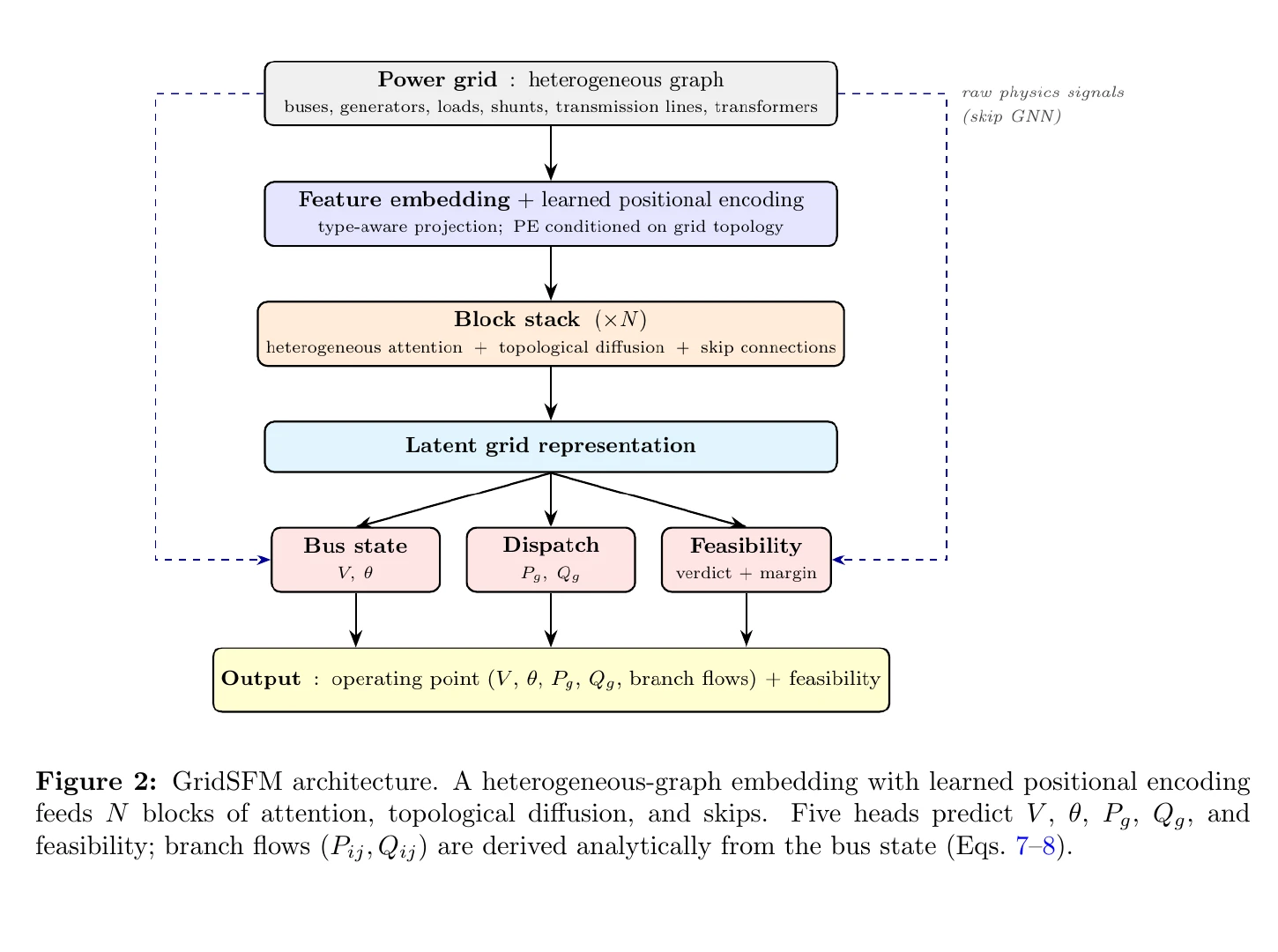
Current designs handle that gap in layers. The model first proposes a state or dispatch. Physics-informed training penalizes violations of the power-flow equations and operating limits. Analytical decoders derive flows from predicted voltages instead of learning every quantity independently. Corrective layers—including DeepOPF's feasibility post-processing—project or iteratively adjust the proposal. A verifier then measures feasibility, objective value, and confidence before the result is accepted, rejected, or passed to a conventional solver as a warm start.

Those layers do different jobs. A physics penalty improves average behavior but is not a hard guarantee. A correction step can repair equality constraints while leaving an engineering limit violated. A feasibility classifier can route cases without proving every continuous constraint. Exact verification can bound worst-case violations over a defined input region, but the verification problem itself becomes difficult as networks and models grow. The system is credible when it states which guarantee comes from which layer.

A transmission system already has the structure a graph neural network expects. Buses become nodes; lines and transformers become edges; generators, loads, limits, costs, and electrical parameters become typed features. Message passing lets the model combine local electrical relationships with wider network context without flattening every grid into one fixed-length vector.

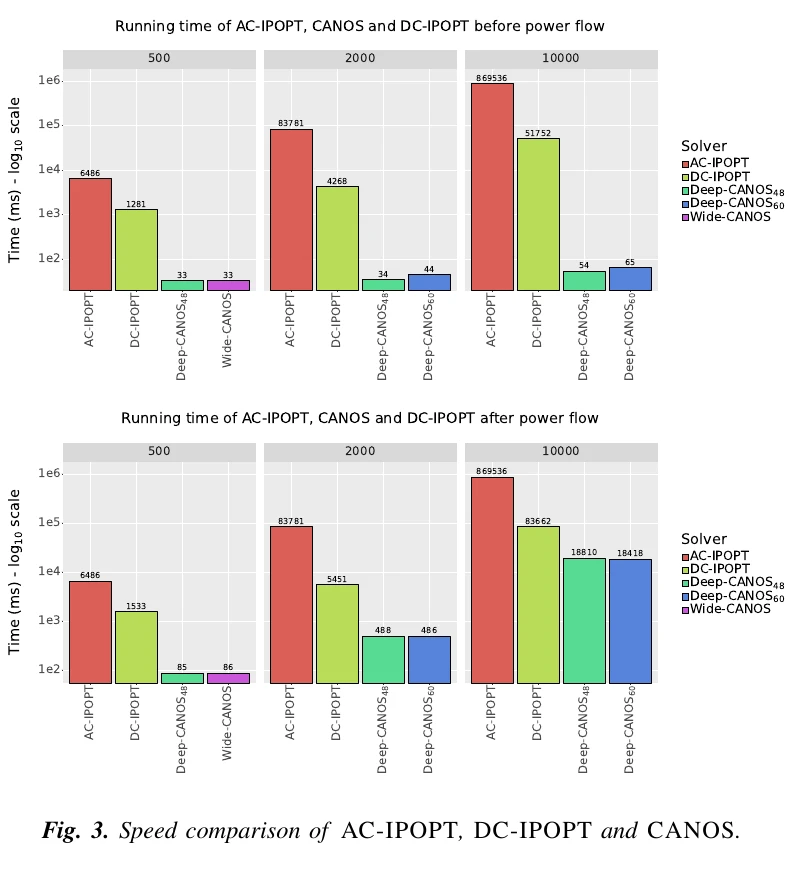
That structure matters when the network changes. CANOS, a graph-based AC-OPF model published in 2024, was evaluated on networks from 500 to 10,000 buses and on single-component, or N-1, topology changes. Its authors reported inference times of 33 to 65 milliseconds and solutions within 1 percent of the reference AC-OPF cost, together with detailed constraint-violation measurements. The result was a large scaling demonstration, not a guarantee of feasibility for every unseen operating condition.

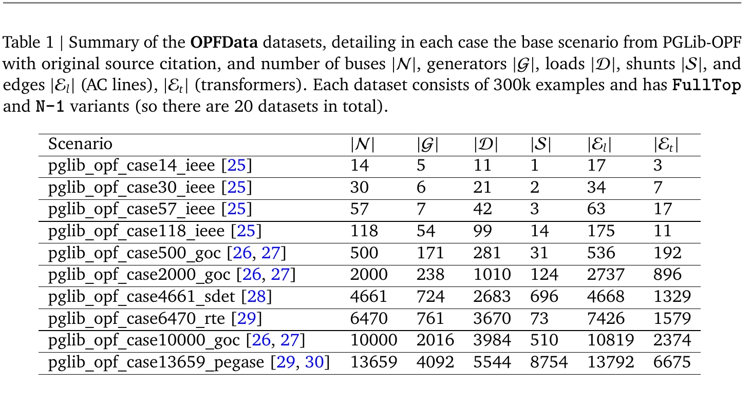
Benchmarks are catching up to that question. The IEEE Power Grid Library standardized AC-OPF formulations and test networks so methods could be compared on the same problems. OPFData later added hundreds of thousands of solved cases per network, grids as large as 13,659 buses, and variants with generator or branch outages. Its own limitations are instructive: synthetic load perturbations and selected outage patterns cover only part of the operating space a utility faces.

A solver benchmark needs at least four axes. Runtime measures how long the online calculation takes, including any correction or fallback. Feasibility measures power balance and every operating constraint, not merely whether the model returned a value. Optimality compares the objective against a defined reference solution. Generalization tests loads, costs, topologies, contingencies, and grids outside the training distribution.

The axes can move against one another. More correction iterations may improve feasibility and reduce the cost gap while giving back some latency. A model can be faster than a full AC solver and still slower than a DC approximation. It can match a reference objective closely while violating a limit the objective does not price. It can perform well on a 10,000-bus benchmark and still need fine-tuning for a different network.

Hardware and stopping rules matter too. A GPU neural model compared with a single CPU solver does not isolate the algorithmic speedup. The classical baseline's initialization, tolerances, parallelism, and convergence criteria can change the result. The useful benchmark reports the full path on disclosed hardware: data preparation, inference, correction, verification, numerical fallback, and the share of cases each stage resolves.

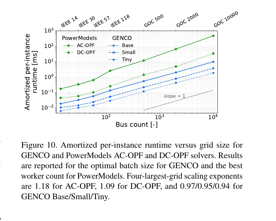
GENCO, released by IBM Research and collaborators in August 2026, uses one geometric graph architecture for power flow, optimal power flow, and state estimation. The authors report tests on grids up to 10,000 buses, up to an 85-fold OPF speedup over the IPOPT interior-point solver with an optimality gap no greater than 0.3 percent in the reported cases, and validation using a year of Hydro-Québec SCADA data on a 1,200-bus network. They also report robustness tests with as many as 20 simultaneous component outages. Zero-shot transfer to an entirely unseen grid remains an open problem in the paper.

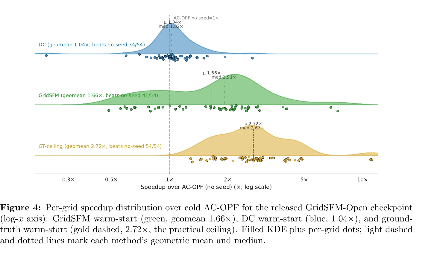
GridSFM, described by Microsoft Research in a May 2026 technical white paper, widens the other axis. It was trained across about 200 grid topologies and more than half a million scenarios, predicts a complete AC-OPF operating point plus a feasibility classification, and can seed a conventional solver. Microsoft reports a 1.66-fold solver acceleration from that warm start and improved adaptation to an unseen grid after fine-tuning on a limited number of cases.

These are author-reported results from a new preprint and a technical white paper, not independent evidence that either model is ready to clear a live market. Their importance is architectural. GENCO asks whether one representation can support several steady-state tasks on a grid. GridSFM asks whether one representation can transfer across many grids. Together they move the research target beyond a separate surrogate trained for every network and every calculation.

The baseline is not a frozen CPU solver. The Exascale Grid Optimization toolkit from Pacific Northwest National Laboratory runs AC optimal power-flow variants across CPUs and GPUs, including stochastic, security-constrained, and multi-period formulations. ARPA-E's second Grid Optimization Competition produced hybrid numerical systems that combine nonlinear optimization, decomposition, contingency screening, parallelism, and heuristics.

One ARPA-E project reported near-optimal solutions for security-constrained AC-OPF cases with as many as 31,000 buses and 1,200 contingencies in five to 60 minutes. That timing is not interchangeable with a millisecond neural inference result: the problem includes far more security and discrete structure. It demonstrates why comparisons must match the formulation before comparing the clock.

The strongest near-term systems are likely to combine both lines of work. A neural model can screen thousands of cases, identify likely active constraints, rank contingencies, or supply a high-quality starting point. The numerical optimizer can enforce the complete formulation on the smaller set that survives. This is less dramatic than replacing the solver and more useful than treating machine learning and mathematical optimization as competing camps.

Planning studies and security assessment create the natural opening because they repeat related calculations at enormous scale. A neural solver can rank contingencies, screen infeasible scenarios, approximate an AC state where a DC model would omit voltage and reactive power, or accelerate the high-fidelity solve that follows. Interconnection analysis can use the same pattern to examine more combinations of load, generation, upgrades, and outages without treating the surrogate as the final study result.

Operations offer narrower paths: warm-starting power flow or OPF, filling a state estimate when a conventional method struggles with sparse measurements, and flagging cases for a full solve. None of those applications turns a steady-state neural solver into transient-stability analysis, protection logic, automatic generation control, or an end-to-end market-clearing system. The deployment boundary should name the task, the input range, the fallback, and the authority that accepts the result.

The next evidence to watch is concrete: independent reproduction on standardized hardware; validation on several real utility networks; exact or conservative feasibility guarantees at AC scale; transfer to unseen topologies without extensive retraining; and integration with security-constrained, multi-period, and discrete decisions. Open benchmark sets such as OPFData make those claims easier to test. When the results arrive together, neural solvers will have advanced from fast approximations of selected cases to a dependable layer in the grid's optimization stack.