Day-ahead vs. real-time electricity prices: why a price spike can erase revenue
A worked ERCOT settlement example for analysts: follow an 80 MWh day-ahead sale through a generation shortfall, a price spike, and the final energy revenue.
October 14, 20266 min read
A generator sells 80 MWh for delivery in an hour at $50/MWh. When that hour arrives, the real-time price is $200/MWh, but the plant produces only 60 MWh. In this hypothetical example, its energy settlement revenue is zero. The higher price makes the shortfall expensive enough to absorb the entire day-ahead sale.
If you are new to a generator’s commercial team, this is a useful first reconciliation. A price chart shows what electricity is worth at a place and time. To explain what the plant earns, you also need the quantity it sold ahead and the quantity it delivered.
Day-ahead prices establish an earlier financial position for delivery. Real-time settlement prices the difference between that position and actual delivery. Work through the two cash flows below, then change the generation and price inputs to see which part of the revenue moves.
What happens when delivery changes?
You sold 80 MWh day-ahead at $50/MWh. Change generation or the real-time price.
Total energy settlement revenue
$0
-20 MWh × $200/MWh = -$4,000 in real-time settlement.
Hypothetical teaching example. Same location and delivery period; excludes other revenues, charges, and costs.
In this article · 5 sections
01
The $4,000 sale and the $4,000 shortfall
In the example, the day-ahead sale earns 80 MWh × $50/MWh = $4,000. The plant then delivers 20 MWh less than it sold. At a constant real-time price of $200/MWh, that deviation produces a −$4,000 adjustment: −20 MWh × $200/MWh. Add the two cash flows and the energy settlement revenue is $0, before operating costs and other charges.
The plant has not sold its 60 MWh twice. Its delivery is accounted for against the earlier position. The unmatched 20 MWh creates the real-time purchase exposure. That is why multiplying actual generation by the real-time price—60 × $200 = $12,000—does not reconstruct this settlement.
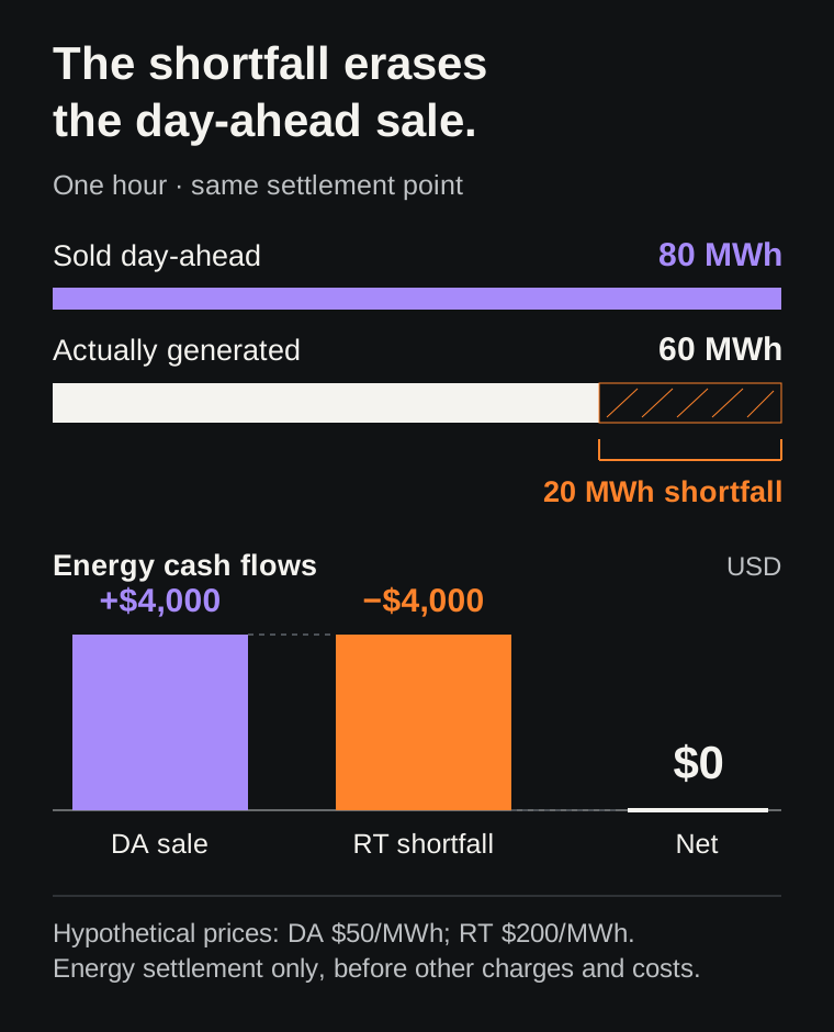
The relationship is: energy revenue = day-ahead MWh × day-ahead price + (actual MWh − day-ahead MWh) × real-time price. Here we hold the location and real-time price constant across the hour to make that relationship visible.
02
The same price produces three different outcomes
Keep the day-ahead sale and both prices unchanged. If the plant delivers exactly 80 MWh, there is no deviation and revenue remains $4,000. If it delivers 100 MWh, the extra 20 MWh earns another $4,000 in real-time settlement. Revenue rises to $8,000.
These are three outcomes under the same price chart. The difference is the plant’s position. A high real-time price helps a generator with extra energy to sell and hurts one that must cover a shortfall.
Negative prices reverse the real-time cash flow. With 60 MWh delivered and a real-time price of −$100/MWh, the −20 MWh deviation creates a positive $2,000 adjustment. The day-ahead sale still earns $4,000, so energy revenue becomes $6,000. Try those inputs in the example; keep the signs attached to both the quantity and the price.
| Actual output | DA sale | RT adjustment | Energy revenue |
|---|---|---|---|
| 60 MWh | $4,000 | −$4,000 | $0 |
| 80 MWh | $4,000 | $0 | $4,000 |
| 100 MWh | $4,000 | +$4,000 | $8,000 |
03
What the two markets are doing
ERCOT’s day-ahead market protocols describe a forward financial market with hourly energy settlement. The day-ahead price is a transaction price for that delivery period, rather than a promise about the later real-time price.
Between the auction and delivery, electricity demand, wind and solar output, available generators, and transmission conditions can change. The real-time system balances conditions as they unfold. A gap between day-ahead and real-time prices tells you the two prices differed; explaining the cause requires the corresponding operating evidence.
For a new analyst, the immediate task is narrower: reconcile the position before explaining the market. You can get the settlement arithmetic right even while the reason for the price spike is still being investigated.
04
Averages can hide the interval that cost the money
Now shrink the sale to 1 MW for one hour, sold day-ahead at $50/MWh. Suppose the plant generates 1 MW for the first three quarter-hours and nothing for the last. The real-time settlement prices are $20, $20, $20, and $200/MWh. These are hypothetical intervals, with constant power inside each interval.
The day-ahead sale earns $50. Delivery matches the allocated sale in the first three intervals. In the last, the plant is short 0.25 MWh: 1 MW × 0.25 hours. Buying that shortfall at $200/MWh costs $50. Energy revenue is again zero.
The simple hourly average price is $65/MWh. Applying it to the 0.25 MWh shortfall would produce a $16.25 charge and a false $33.75 revenue figure. The missing energy occurred entirely in the expensive quarter-hour; an average price loses that fact.
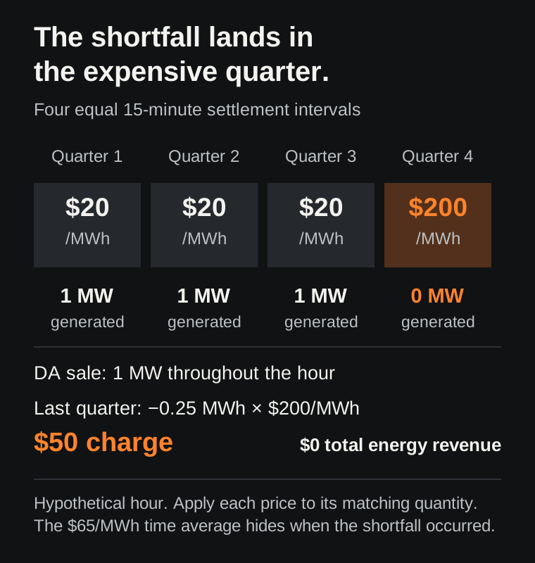
ERCOT’s real-time protocols distinguish dispatch locational marginal prices from 15-minute settlement point prices. Use the settlement product that matches the calculation. Preserve the interval labels and daylight-saving identifiers when joining hourly and quarter-hourly records.
05
Build a reconciliation you can explain to the commercial team
Start with the exact settlement point and operating day. ERCOT publishes day-ahead settlement point prices and the real-time settlement point price product linked below. Pair those prices with the team’s actual day-ahead position and metered generation; public price files alone do not contain a plant’s commercial position.
For each delivery interval, keep five fields together: day-ahead MWh, day-ahead price, actual MWh, deviation MWh, and real-time settlement point price. Calculate the two cash flows separately before summing them. Retain the source version because price corrections and resettlement can change a later reconciliation.
The output should let a colleague trace a revenue change to a price, a quantity, or both. If the hedge references a hub while the generator settles at a node, add that location difference as another calculation. The worked example here deliberately uses one location.
A power buyer can use the same logic with purchases and consumption: buying 80 MWh at $50/MWh and consuming 100 MWh at a constant $200/MWh real-time price costs $8,000 for energy. The retail contract determines how that exposure reaches the customer. For a generator’s next commercial check, read how node-to-hub basis survives a hedge.